Tutorial 4: Human Breast Cancer Dataset

This tutorial illustrates how to apply S3RL to the Human Breast Cancer dataset from 10X Genomics (Visium platform). The dataset can be accessed at 10X Genomics Portal, and includes gene expression, spatial coordinates, and H&E-stained images.

After preprocessing, S3RL enhances the spatial gene expression structure and reveals distinct tissue compartments such as tumor, stromal, and immune-rich regions. Spatial patterns of key marker genes like CXCL14 and DDR1 become more sharply localized, aiding in tumor microenvironment analysis.

import scanpy as sc
import os
import cv2
from S3RL.process_data import process_data
import pandas as pd
import numpy as np

path = '../Data'
dataset = 'Human_Breast_Cancer'
id = ''
knn = 5
pixel_size = 10
path_semantic_fea = '../Img_encoder/models/'

adata = sc.read_h5ad(os.path.join(path, dataset, id, 'sampledata.h5ad'))
adata.var_names_make_unique()

sc.pp.highly_variable_genes(adata, flavor="seurat_v3", n_top_genes=3000, check_values=False)
sc.pp.normalize_total(adata, target_sum=1e4)
sc.pp.log1p(adata)

Ann_df = pd.read_csv(os.path.join(path, dataset, id, 'annotation.txt'), sep='\t', header=None, index_col=0)
Ann_df.columns = ['Ground Truth']
drop = Ann_df.loc[adata.obs_names, 'Ground Truth'].isna()
adata = adata[~drop]
adata = adata[:, adata.var['highly_variable']]

image = cv2.imread(os.path.join(path, dataset, id, 'spatial/tissue_hires_image.png'))
semantic_fea = np.load(os.path.join(path_semantic_fea, dataset, id, 'img_emb.npy'))

adata = process_data(adata, image, pixel=pixel_size, knn=knn, semantic_fea=semantic_fea)

from S3RL.model import S3RL
import yaml
import torch
from sklearn.metrics import adjusted_rand_score

device = torch.device("cuda:0")
C = len(set(Ann_df[Ann_df['Ground Truth'].notna()]['Ground Truth'].values.tolist()))
cfg_path = './Best_cfg'
with open(os.path.join(cfg_path, dataset, dataset+'.yaml'), 'r') as f:
    cfg = yaml.safe_load(f)

model = S3RL(adata, n_clu=C, device=device, **cfg)

adata = model.train()

Training the S3RL model:  93%|█████████▎| 1388/1500 [01:12<00:05, 19.13it/s]

Reached the tolerance, early stop training at epoch 1388

adata.obs['Ground Truth'] = Ann_df.loc[adata.obs_names, 'Ground Truth']
ground_truth = adata.obs['Ground Truth'].astype('category').cat.codes.values
print('ARI is', adjusted_rand_score(ground_truth, adata.obs['pred']))

ARI is 0.672327896923898

import matplotlib
from S3RL.tools import hungarian_match
import numpy as np
import matplotlib.pyplot as plt

label_pred = hungarian_match(ground_truth, adata.obs['pred'])
label_dict = dict(zip(ground_truth, adata.obs['Ground Truth'].values))

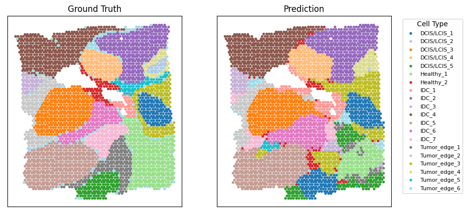
fig, axs = plt.subplots(1, 2, figsize=(10, 5))

colors = np.vstack([np.array(matplotlib.colormaps['tab20'].colors),
                    np.array(matplotlib.colormaps['tab20b'].colors),
                    np.array(matplotlib.colormaps['tab20c'].colors)])

for i in set(ground_truth):
    axs[0].scatter(adata.obsm['spatial'][ground_truth==i, 0], adata.obsm['spatial'][ground_truth==i, 1], color=colors[i], s=8)
    axs[1].scatter(adata.obsm['spatial'][label_pred==i, 0], adata.obsm['spatial'][label_pred==i, 1], color=colors[i], s=8, label=label_dict[i])

axs[1].legend(bbox_to_anchor=(1.05, 1), loc='upper left', fontsize=8, title='Cell Type', title_fontsize=10)
axs[0].set_xticks([])
axs[0].set_yticks([])
axs[1].set_xticks([])
axs[1].set_yticks([])

axs[0].set_title('Ground Truth')
axs[1].set_title('Prediction')

plt.show()